Syllabus:

Multicompartment models: Two compartment open model. I.V bolus Kinetics of multiple dosing, steady state drug levels, calculation of loading and maintenance doses and their significance in clinical settings.

MULTICOMPARTMENT MODELS- (Delayed Distribution Models)

• One-compartment model adequately describes pharmacokinetics of many drugs. Instantaneous distribution equilibrium is assumed in such cases and decline in the amount of drug in the body with time is expressed by an equation with a monoexponential term (i.e. elimination). 
• However, instantaneous distribution is not truly possible for an even larger number of drugs and drug disposition is not monoexponential but bi- or multi-exponential. 
• This is because the body is composed of a heterogeneous group of tissues each with different degree of blood flow and affinity for drug and therefore different rates of equilibration. Ideally, a true pharmacokinetic model should be the one with a rate constant for each tissue undergoing equilibrium, which is difficult mathematically.
• Multicompartment models arethus based on following assumptions –
  1. Blood/plasma and the highly perfused tissues such as tissues such as brain, heart, lung, liver and kidneys constitute the central compartment.
  2. Other tissues with similar distribution characteristics are pooled together to constitute peripheral compartments tissues on the basis of similarity in their distribution characteristics.
  3. Intravenously administered medications are introduced directly into the central compartment.
  4. Irreversible drug elimination, either by hepatic biotransformation or renal excretion, takes place only from the central compartment.
  5. Reversible distribution occurs between central and peripheral compartments, with a finite time required for distribution equilibrium to be attained.
  6. After drug equilibration between drug and the peripheral compartments, elimination of drug follows first-order kinetics.
  7. All rate processes involving passage of drug in and out of individual compartment are first-order processes and plasma level-time curve is best described by sum of series of exponential terms each corresponding to first-order rate processes associated with a given compartment.
  8. The peripheral compartment is usually inaccessible to direct measurement and is not a site of drug elimination or clearance.

TWO-COMPARTMENT OPEN MODEL

• The commonest of all multicompartment models is a two-compartment model. In such a model, the body tissues are broadly classified into 2 categories –
  1. Central Compartment or Compartment 1 comprising of blood and highly perfused tissues like liver, lungs, kidneys, etc. that equilibrate with the drug rapidly. Elimination usually occurs from this compartment.
  2. Peripheral or Tissue Compartment or Compartment 2 comprising of poorlyperfused and slow equilibrating tissues such as muscles, skin, adipose, etc. and considered as a hybrid of several functional physiologic units.
• Classification of a particular tissue, for example brain, into central or peripheral compartment depends upon the physicochemical properties of the drug. A highly lipophilic drug can cross the BBB and brain would then be included in the central compartment. In contrast, a polar drug cannot penetrate the BBB and brain in this case will be a part of peripheral compartment despite the fact that it is a highly perfused organ.
• The plasma concentration for a drug that follows a two-compartment model declines biexponentially as the sum of two first-order processes – distribution and elimination.
• Depending upon the compartment from which the drug is eliminated, the two-compartment model can be categorized into 3 types:
  1. Two-compartment model with elimination from central compartment.
  2. Two-compartment model with elimination from peripheral compartment.
  3. Two-compartment model with elimination from both the compartments.

In the absence of information, elimination is assumed to occur exclusively from central compartment.

Two-Compartment Open Model

Intravenous Bolus Administration

• The model can be depicted as shown below with elimination from the central compartment.

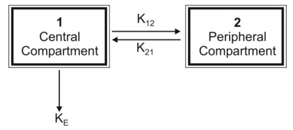
• After the i.v. bolus of a drug that follows two-compartment kinetics, the decline in plasma concentration is biexponential indicating the presence of two disposition processes viz. distribution and elimination. 
• These two processes are not evident to the eyes in a regulararithmetic plot but when a semilog plot of C versus t is made, they can be identified (Fig. 9.12). 
• Initially, the concentration of drug in the central compartment declines rapidly; this is due to the distribution of drug from the central compartment to the peripheral compartment. The phase during which this occurs is therefore called as the distributive phase. 
• After sometime, a pseudo-distribution equilibrium is achieved between the two compartments following which the subsequent loss of drug from the central compartment is slow and mainly due to elimination. This second, slower rate process is called as the post-distributive or elimination phase. 
• In contrast to the central compartment, the drugconcentration in the peripheral compartment first increases and reaches a maximum. This corresponds with the distribution phase. Following peak, the drug concentration declines which corresponds to the post-distributive phase (Fig.9.12).

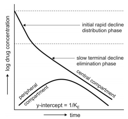
Fig. 9.12. Changes in drug concentration in the central (plasma) and the peripheralcompartment after i.v. bolus of a drug that fits two-compartment model.

• Let K₁₂ and K₂₁ be the first-order distribution rate constants depicting drug transfer between the central and the peripheral compartments and let subscript c and p define central and peripheral compartment respectively. 
• The rate of change in drug concentration in the central compartment is given by:

• Extending the relationship X = V_dC to the above equation, we have

where X_c and X_p are the amounts of drug in the central and peripheral compartments respectively and V_c and V_p are the apparent volumes of the central and the peripheral compartment respectively. 

• The rate of change in drug concentration in the peripheral compartment is given by:

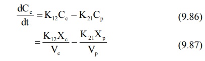
• Integration of equations 9.85 and 9.87 yields equations that describe the concentration of drug in the central and peripheral compartments at any given time t:

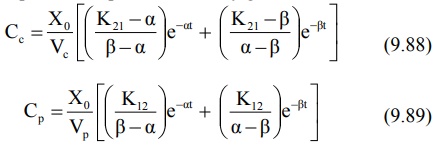
where X_o = i.v. bolus dose, α and β are hybrid first-order constants for the rapid distribution phase and the slow elimination phase respectively which depend entirely upon the first-order constants K₁₂, K₂₁ and K_E.

• The constants K₁₂andK₂₁ that depict reversible transfer of drug between compartments are called as transfer constants or microconstants.
• The mathematical relationshipsbetween hybrid and transfer constants are given as:

α + β = K₁₂ + K₂₁ + K_E                     (9.90)

αβ = K₂₁K_E                    (9.91)

Equation 9.88 can be written in simplified form as:

C_c = Ae ^–αt + Be ^βt                (9.92)

C_c = Distribution exponent Elimination exponent

where A and B are also hybrid constants for the two exponents and can be resolved graphically by the method of residuals.

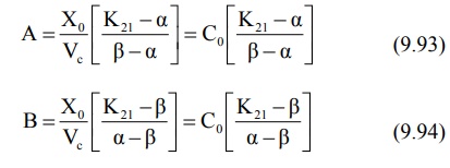
where C_o = plasma drug concentration immediately after i.v. injection.

Method of Residuals: The biexponential disposition curve obtained after i.v. bolus of adrug that fits two compartment model can be resolved into its individual exponents by the method of residuals. Rewriting the equation 9.92:

C_c = Ae ^-αα + Be ^-βt                     (9.92)

As apparent from the biexponential curve given in Fig. 9.12., the initial decline due to distribution is more rapid than the terminal decline due to elimination i.e. the rate constant α >> ß and hence the term e^–αt approaches zero much faster than does e^–βt. Thus, equation 9.92 reduces to:

In log form, the equation

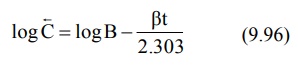
where C = back extrapolated plasma concentration values. A semilog plot of C versus t yields the terminal linear phase of the curve having slope –β/2.303 and when back extrapolated to time zero, yields y-intercept log B (Fig. 9.13.).The t_½ for the elimination phase can be obtained from equation t_½ = 0.693/β.

Subtraction of extrapolated plasma concentration values of the elimination phase (equation 9.95) from the corresponding true plasma concentration values (equation 9.92) yields a series of residual concentration values C_r.

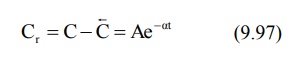
In log form, the equation becomes:

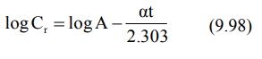
A semilog plot of C_r versus t yields a straight line with slope –α/2.303 and Y-intercept log A (Fig. 9.13).

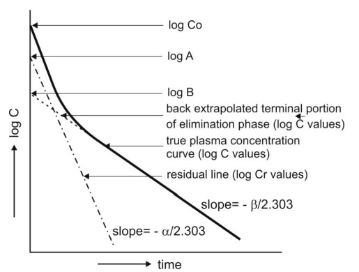
Fig. 9.13. Resolution of biexponential plasma concentration-time curve by the method of residuals for a drug that follows two-compartment kinetics on i.v. bolus administration.

KINETICS OF MULTIPLE DOSING

DESIGN OF DOSAGE REGIMENS

• Dosage regimen is defined as the manner in which a drug is taken. 
• For some drugs likeanalgesics, hypnotics, antiemetics, etc., a single dose may provide effective treatment.
• However, the duration of most illnesses is longer than the therapeutic effect produced by a single dose. In such cases, drugs are required to be taken on a repetitive basis over a period of time depending upon the nature of illness. Thus, for successful therapy, design of an optimal multiple dosage regimen is necessary.
• An optimal multiple dosage regimen is the one in which the drug is administered in suitable doses (by a suitable route), with sufficient frequency that ensures maintenance of plasma concentration within the therapeutic window (without excessive fluctuations and drug accumulation) for the entire duration of therapy.For some drugs like antibiotics, a minimum effective concentration should be maintained at all times and for drugs with narrow therapeutic indices like phenytoin, attempt should be made not to exceed toxic concentration.

Approaches to Design of Dosage Regimen

• The various approaches employed in designing a dosage regimen are –
  1. Empirical Dosage Regimen –is designed by the physician based on empirical clinicaldata, personal experience and clinical observations. This approach is, however, not very accurate.
  2. Individualized Dosage Regimen –is the most accurate approach and is based on thepharmacokinetics of drug in the individual patient. The approach is suitable for hospitalised patients but is quite expensive.
  3. Dosage Regimen on Population Averages –This is the most often used approach.The method is based on one of the two models –
     • (a) Fixed model –here, population average pharmacokinetic parameters are used directly to calculate the dosage regimen.
     • (b) Adaptive model –is based on both population average pharmacokinetic parameters of the drug as well as patient variables such as weight, age, sex, body surface area and known patient pathophysiology such as renal disease.
• Irrespective of the route of administration and complexity of pharmacokinetic equations, the two major parameters that can be adjusted in developing a dosage regimen are —
• The dose size — the quantity of drug administered each time, and
• The dosing frequency — the time interval between doses.
• Both parameters govern the amount of drug in the body at any given time. 

Dose Size

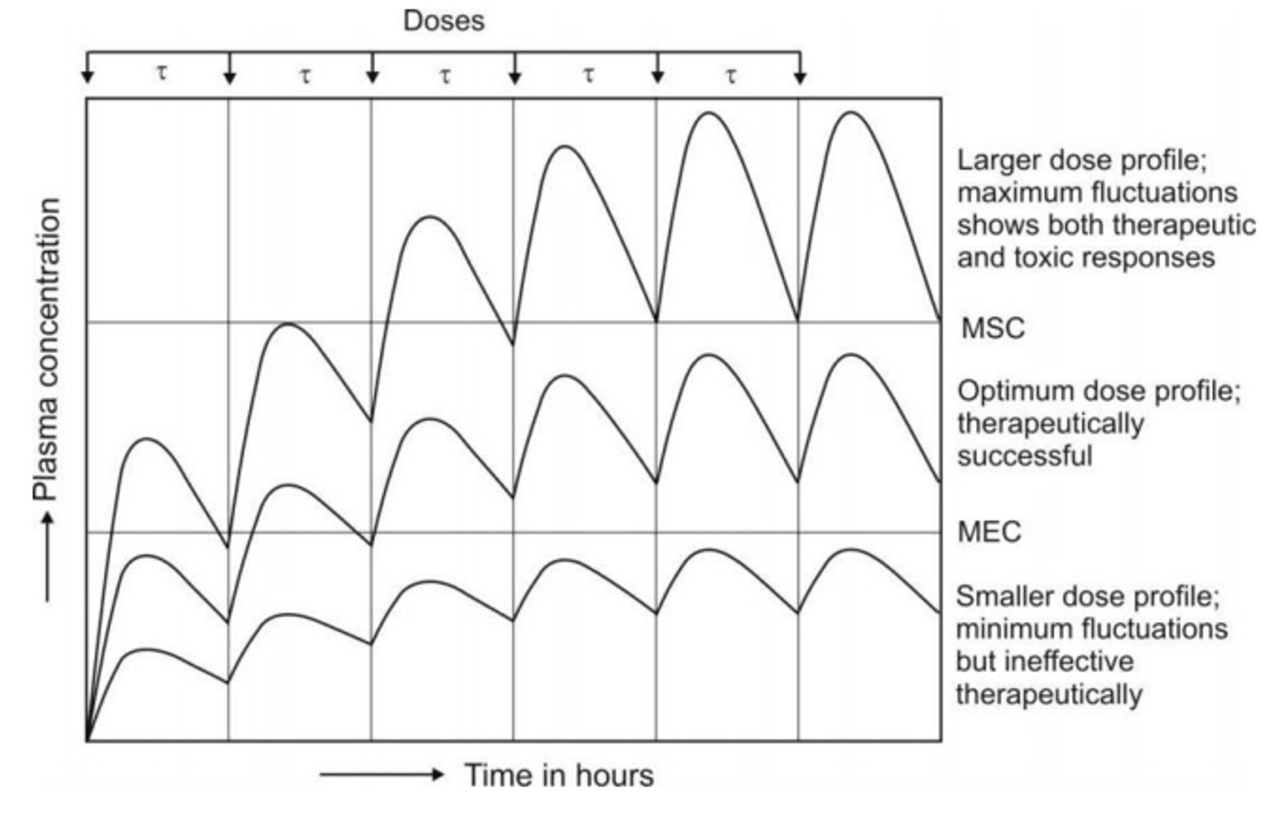
• The magnitude of both therapeutic and toxic responses depends upon dose size.
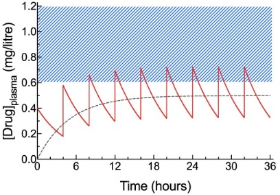
• Dose size calculation also requires the knowledge of amount of drug absorbed after administration of each dose. Greater the dose size, greater the fluctuations between C_ss,max and C_ss,min during each dosing interval and greater the chances of toxicity (Fig. 12.1).
• For drugs administered chronically, dose size calculation is based on average steady state blood levels and is computed from equation 12.8.

Dosing Frequency

• The dose interval (inverse of dosing frequency) is calculated on the basis of half-life of the drug. 
• If the interval is increased and the dose is unchanged, C_max, C_min and C_av decrease but the ratio C_max/C_min increases. Opposite is observed when dosing interval is reduced or dosing frequency increased. It also results in greater drug accumulation in the body and toxicity (Fig. 12.2).

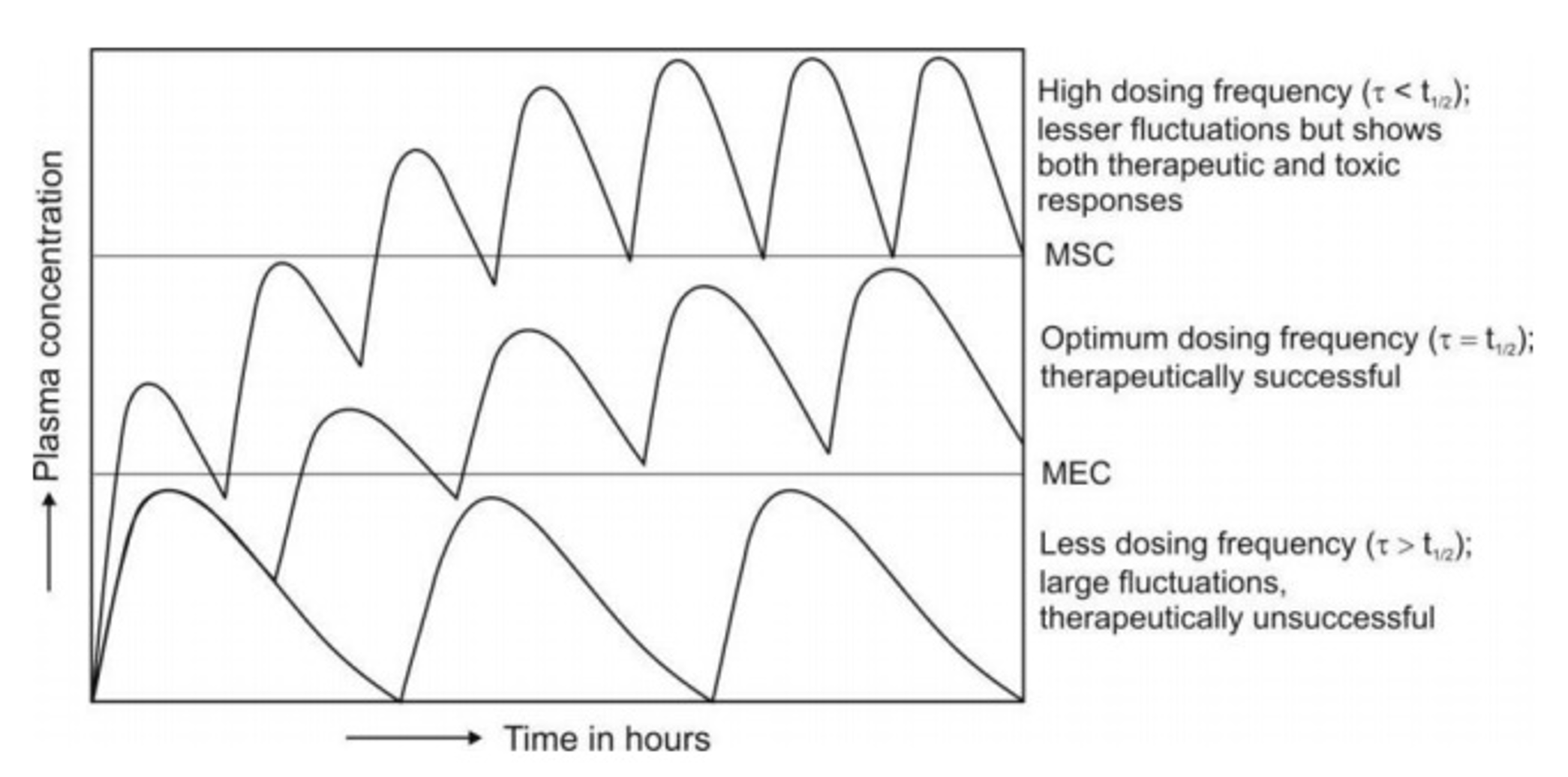
• A proper balance between both dose size and dosing frequency is often desired to attain steady-state concentration with minimum fluctuations and to ensure therapeutic efficacy and safety. The same cannot be obtained by giving larger doses less frequently. However, administering smaller doses more frequently results in smaller fluctuations.
• Generally speaking, every subsequent dose should be administered at an interval equal to half-life of the drug. A rule of thumb is that –
  • For drugs with wide therapeutic index such as penicillin, larger doses may be administered at relatively longer intervals (more than the half-life of drug) without any toxicity problem^.
  • For drugs with narrow therapeutic index such as digoxin, small doses at frequent intervals (usually less than the half-life of the drug) is better to obtain a profilewith least fluctuations which is similar to that observed with constant rate infusion or controlled-release system.

Drug Accumulation During Multiple Dosing

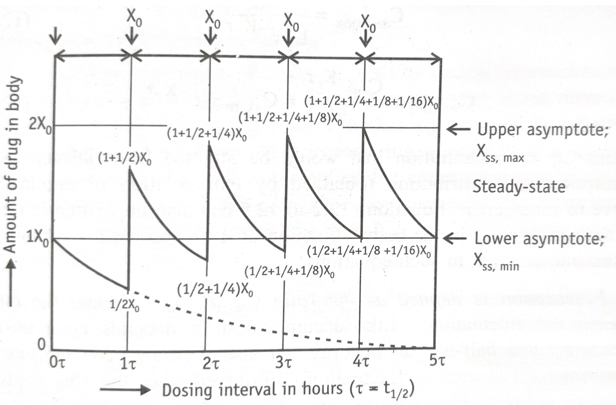
• Consider the amount of drug in the body-time profile shown in Fig. 12.3. obtained after i.v. multiple dosing with dosing interval equal to one t_½.
• After the administration of first dose X_o at τ = 0, the amount of drug in the body will be X = 1X_o.
• At the next dosing interval when X = ½X_o, the amount of drug remaining in the body, administration of the next i.v. dose raises the body content to X = X_o + ½X_o i.e. drug accumulation occurs in the body.
• Thus, accumulation occurs because drug from previous doses has not been removed completely. As the amount of drug in the body rises graduallydue to accumulation, the rate of elimination also rises proportionally until a steady-state or plateau is reached when the rate of drug entry into the body equals the rate of exit.
• The maximum and minimum values of X i.e. X_ss,max and X_ss,min approach respective asymptotes at plateau.
• It is interesting to note that at plateau, X_ss,min = 1X_o and X_ss,max = 2X_o i.e. X_ss,min equals the amount of drug in the body after the first dose and X_ss,max equals twice the first dose. Also (X_ss,max – X_ss,min) = X_o and X_ss,max/X_ss,min = 2. All this applies only when τ  = t_½ and drug is administered intravenously. When τ < t_½, the degree of accumulation is greater and vice-versa.
• Thus, the extent to which a drug accumulates in the body during multiple dosing is independent of dose size, and is a function of –
  • Dosing interval, and
  • Elimination half-life.
• The extent to which a drug will accumulate with any dosing interval in a patient can be derived from information obtained with a single dose and is given by accumulation index R_ac as:

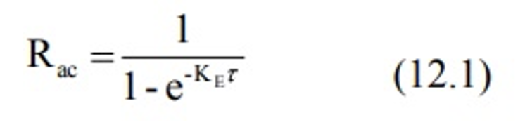
Understanding (R_ac) Values

• (R_ac) = 1 : No accumulation (the drug is fully eliminated before the next dose).
• (R_ac) > 1 : Accumulation occurs (the drug concentration builds up until it reaches a plateau, or steady-state).

Time to Reach Steady-State During Multiple Dosing

• The Process: After each dose, the amount of drug in your body increases. However, the body naturally clears more of the drug as the concentration rises.
• Dynamic Balance: Eventually, these two forces—input and elimination—equalize. Even though drug levels fluctuate slightly between doses (rising to a peak and falling to a low), the average concentration remains constant. 
• It means “A steady-state drug level occurs when the rate of a drug entering your body matches the rate of the drug being eliminated.” At this point, the overall concentration of the medication remains stable.
• To maintain the drug within a safe and effective therapeutic range during repeated dosing, the doses should be given at t_1/2 of a drug. 
• The time required to reach steady-state depends primarily upon the half-life of the drug. Provided K_a >> K_E, the plateau is reached in approximately 5 half-lives. This is called as plateau principle.
• It also means that the rate at which the multiple dose steady-state isreached is determined only by K_E.
• The time taken to reach steady-state is independent of dose size, dosing interval and number of doses.

Maximum and Minimum Concentration During Multiple Dosing

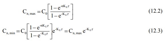
• If n is the number of doses administered, the C_max and C_min obtained on multiple dosing after the n^th dose is given as:

• The maximum and minimum concentration of drug in plasma at steady-state are found by following equations:

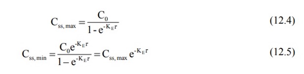
where C_o = concentration that would be attained from instantaneous absorption and distribution (obtained by extrapolation of elimination curve to time zero). Equations 12.2 to 12.5 can also be written in terms of amount of drug in the body. Fraction of dose absorbed, F, should be taken into account in such equations.

• Fluctuation is defined as the ratio C_max/C_min. Greater the ratio, greater the fluctuation.Like accumulation, it depends upon dosing frequency and half-life of the drug. It also depends upon the rate of absorption. The greatest fluctuation is observed when the drug is given as i.v. bolus. Fluctuations are small when the drug is given extravascularly because of continuous absorption.

Average Concentration and Body Content on Multiple Dosing to Steady-State 

The average drug concentration at steady-state C_ss,av is a function of –

• The maintenance dose X_o,
• The fraction of dose absorbed F,
• The dosing interval τ and
• Clearance Cl_T (or V_d and K_E or t_½) of the drug.

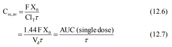
where the coefficient 1.44 is the reciprocal of 0.693 in equation 12.7. AUC is the area under the curve following a single maintenance dose. Equation 12.7 can be used to calculate maintenance dose of a drug to achieve a desired concentration. Since X = V_d C, the body content at steady-state is given as:

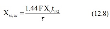
These average values are not arithmetic mean of C_ss,max and C_ss,min since the plasma drug concentration declines exponentially.

Calculation of Loading and Maintenance Doses

• A loading dose is a large initial dose of medication given to rapidly achieve therapeutic drug levels in the body.
• A maintenance dose is the smaller, regular dose given afterward to sustain that therapeutic level over time. 
• A drug does not show therapeutic activity unless it’s concentration crosses the minimum effective concentration (MEC).
• To get a constant therapeutic effect, the concentration of drug should be in a therapeutic window and should reach the desired steady-state in therapeutic window only. 
• It takes about 5 half-lives to attain the steady state and therefore the time taken will be too long if the drug has a long half-life. Plateau can be reached immediately by administering a dose that gives the desired steady-state instantaneously before the commencement of maintenance doses X_o (second dose or subsequent dose).
• Such an initial or first dose intended to be therapeutic is called as priming dose orloadingdose X_o,L. A simple equation for calculating loading dose is:

• For i.v loading dose,

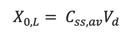
• For e.v loading dose,

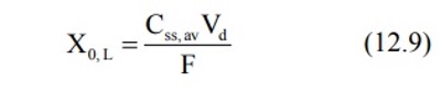
Where,
X_o,L – Loading dose.
C_ss,av – Average concentration at steady state.
V_d – Volume of distribution.

• After e.v. administration, C_max is always smaller than that after i.v. administration.
• For drugs having low therapeutic indices, the loading dose may be divided into smaller doses to be given at various intervals before the first maintenance dose.
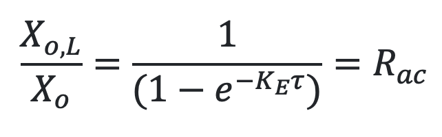
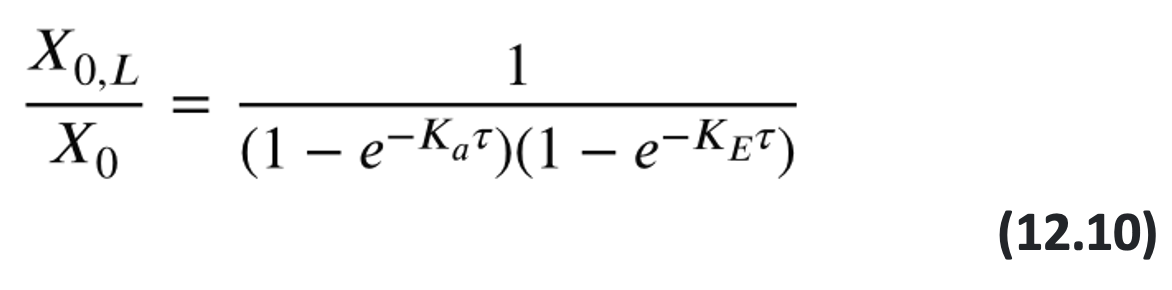
• When V_d is not known, loading dose may be calculated by the following equation:

• For i.v administration:

• For e.v administration:

Where,
X_oL – Loading dose
X_o – Maintenance dose

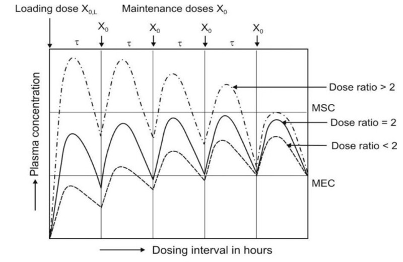
• The ratio of loading dose to maintenance dose X_o,L/X_ois called as dose ratio.
  • As a rule,when τ = t_½, dose ratio should be equal to 2.0.
  • when τ  > t_½, dose ratio must be smaller than 2.0 and
  • when τ < t_½, dose ratio must be greater than 2.0.

Fig. 12.4. shows that if loading dose is not optimum, either too low or too high, the steady-state is attained within approximately 5 half-lives in a manner similar to when no loading dose is given.

Maintenance of Drug within the Therapeutic Range

The ease or difficulty in maintaining drug concentration within the therapeutic window depends upon —

1. The therapeutic index of the drug
2. The half-life of the drug
3. Convenience of dosing.

It is extremely difficult to maintain such a level for a drug with short half-life (less than 3 hours) and narrow therapeutic index e.g. heparin, since the dosing frequency has to be essentially less than t_½. However, drugs such as penicillin (t_½ = 0.9 hours) with high therapeutic index may be given less frequently (every 4 to 6 hours) but the maintenance dose has to be larger so that the plasma concentration persists above the minimum inhibitory level.

A drug with intermediate t_½ (3 to 8 hours) may be given at intervals τ ≤ t_½ if therapeutic index is low and those with high indices can be given at intervals between 1 to 3 half-lives. Drugs with half-lives greater than 8 hours are more convenient to dose. Such drugs are usually administered once every half-life. Steady-state in such cases can be attained rapidly by administering a loading dose. For drugs with very long half-lives (above 24 hours) e.g. amlodipine, once daily dose is very convenient.

Core Differences

Feature	Loading Dose	Maintenance Dose
Purpose	To reach the target drug concentration in the body immediately.	To keep the drug concentration stable within the therapeutic window.
Timing	Administered once or over a short period at the start of treatment.	Taken continuously (e.g., daily) or at regular intervals (e.g., every 8 hours).
Dosage Size	Larger (often substantially higher than the maintenance dose).	Smaller (tailored to how fast the drug is eliminated from the body).
Why it’s needed	Essential for drugs that take a long time to build up to effective levels on their own.	Replaces the drug that is naturally metabolized and excreted by the body.

Significance of Loading dose and Maintenance dose

The Significance of a Loading Dose

• Rapid Onset of Action: Drugs that are slowly eliminated from the body (those with a long half-life) can take days or weeks to reach an effective therapeutic level if only standard doses are used. A loading dose bypasses this delay. 
• Critical Situations: It is highly significant in acute, life-threatening conditions where immediate clinical effects are necessary (e.g., administering antiarrhythmics for heart conditions, antibiotics for severe infections, or anticonvulsants to stop seizures). 

The Significance of a Maintenance Dose

• Sustaining Therapeutic Levels: Once the target level is established by the loading dose, maintenance doses are given to compensate exactly for the amount of drug the body eliminates or metabolizes over time.
• Preventing Toxicity:  The rate of a maintenance dose is determined by the drug’s clearance rate(how fast the body removes the drug) and its bioavailability.

---