Unit-III: Pharmacokinetics

Syllabus

Pharmacokinetics: Definition and introduction to Pharmacokinetics, Compartment models, Non-compartment models, physiological models, One compartment open model – (a). Intravenous Injection (Bolus) (b). Intravenous infusion and (c) Extra vascular administrations. Pharmacokinetics parameters – K_E, t_1/2, V_d, AUC, K_a, Cl_t and CL_R– definitions methods of eliminations, understanding of their significance and application.

---

Pharmacokinetics: Definition and Introduction to Pharmacokinetics

• The duration of drug therapy ranges from a single dose of a drug taken for relieving an acute condition such as headache to drugs taken life-long for chronic conditions such as hypertension, diabetes, asthma or epilepsy. 
• Dosage regimen = Dose + Administration Frequency
• The frequency of administration of a drug in a particular dose is called as dosage regimen.
• Depending upon the therapeutic objectiveto be attained, the duration of drug therapy and the dosage regimen are decided.
• The drug fails to elicit a therapeutic response when the concentration is below the effective level and precipitates adverse reactions when above the toxic level. The plasma drug concentration between these two limits is called as the therapeutic concentration range or therapeutic window.
• The ratio of maximum safe concentration to minimum effective concentration of the drug is called as the therapeutic index. 
• Pharmacokinetics is defined as the kinetics of drug absorption, distribution, metabolism and excretion (KADME) and their relationship with the pharmacological, therapeutic or toxicological response in Human and animals. There are two aspects of pharmacokinetic studies –
  • Theoretical aspect –which involves development of pharmacokinetic models topredict drug disposition after its administration. Statistical methods are commonly applied to interpret data and assess various parameters.
  • Experimental aspect –which involves development of biological samplingtechniques, analytical methods for measurement of drug (and metabolites) concentration in biological samples and data collection and evaluation.
    Several relevant terms can now be defined –
    • Clinical Pharmacokinetics is defined as the application of pharmacokinetic principles in the safe and effective management of individual patient.
    • Population Pharmacokinetics is defined as the study of pharmacokinetic differences of drugs in various population groups.
    • Toxicokinetics is defined as the application of pharmacokinetic principles to the design, conduct and interpretation of drug safety evaluation studies.

Plasma Drug Concentration-Time Profile

• A direct relationship exists between the concentration of drug at the biophase (site of action) and the concentration of drug in plasma. 
• Two categories of parameters can be evaluated from a plasma concentration time profile –
  • Pharmacokinetic parameters, and
  • Pharmacodynamic parameters.
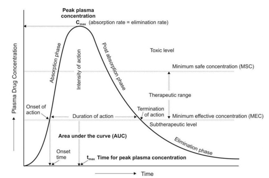
• A typical plasma drug concentration-time curve obtained after a single oral dose of a drug and showing various pharmacokinetic and pharmacodynamic parameters is depicted in Fig. 01. Such a profile can be obtained by measuring the concentration of drug in plasma samples taken at various intervals of time after administration of a dosage form and plotting the concentration of drug in plasma (Y-axis) versus the corresponding time at which the plasma sample was collected (X-axis).

Pharmacokinetic Parameters

The three important pharmacokinetic parameters that describe the plasma level-time curve and useful in assessing the bioavailability of a drug from its formulation are –

1. Peak Plasma Concentration (C_max)
   • The point of maximum concentration of drug in plasma is called as the peak and the concentration of drug at peak is known as peak plasma concentration. It is also calledas peak height concentration and maximum drug concentration. C_max is expressed in mcg/mL. The peak plasma level depends upon –
     • The administered dose
     • Rate of absorption, and
     • Rate of elimination.
   • The peak represents the point of time when absorption rate equals elimination rate of drug. The portion of curve to the left of peak represents absorption phase i.e. when the rate of absorption is greater than the rate of elimination. The section of curve to the right of peak generally represents elimination phase i.e. when the rate of elimination exceeds rate of absorption.
   • Peak concentration is often related to the intensity of pharmacological response and should ideally be above minimum effective concentration (MEC) but less than the maximum safe concentration (MSC).
2. Time of Peak Concentration (t_max)
   • The time for drug to reach peak concentration in plasma (after extravascular administration) is called as the time of peak concentration. It is expressed in hours andis useful in estimating the rate of absorption.
   • Onset time and onset of action are dependent upon t_max. This parameter is of particular importance in assessing the efficacy of drugs used to treat acute conditions like pain and insomnia which can be treated by a single dose.
3. Area Under the Curve (AUC)
   • It represents the total integrated area under the plasma level-time profile and expresses the total amount of drug that comes into the systemic circulation after its administration. AUC is expressed in mcg/mL X hours.
   • It is the most important parameterin evaluating the bioavailability of a drug from its dosage form as it represents the extent of absorption. AUC is also important for drugs that are administered repetitively for the treatment of chronic conditions like asthma or epilepsy.

Pharmacodynamic Parameters

The various pharmacodynamic parameters are –

1. Minimum Effective Concentration (MEC)
   • It is defined as the minimum concentration of drug in plasma required to produce the therapeutic effect. It reflects the minimum concentration of drug at the receptor site toelicit the desired pharmacological response. The concentration of drug below MEC is said to be in the sub-therapeutic level.
   • In case of antibiotics, the term minimum inhibitory concentration (MIC) is used. It describes the minimum concentration of antibiotic in plasma required to kill or inhibit the growth of microorganisms.
2. Maximum Safe Concentration (MSC)
   • Also called as minimum toxic concentration (MTC), it is the concentration of drug in plasma above which adverse or unwanted effects are precipitated. Concentration of drug above MSC is said to be in the toxic level.
3. Onset of Action
   • The beginning of pharmacological response is called as onset of action. It occurswhen the plasma drug concentration just exceeds the required MEC.
4. Onset Time
   • It is the time required for the drug to start producing pharmacological response. Itcorresponds to the time for the plasma concentration to reach MEC after administration of drug.
5. Duration of Action
   • The time period for which the plasma concentration of drug remains above the MEC level is called as duration of drug action. It is also defined as the difference betweenonset time and time for the drug to decline back to MEC.
6. Intensity of Action
   • It is the maximum pharmacological response produced by the peak plasma concentration of drug. It is also called aspeak response.
7. Therapeutic Range
   • The drug concentration between MEC and MSC represents the therapeutic range. Itis also known as therapeutic window.
8. Therapeutic Index
   • The ratio of MSC to MEC is called as therapeutic index. It is also defined as the ratio of dose required to produce toxic or lethal effects to dose required to produce therapeutic effect.

PHARMACOKINETIC ANALYSIS OF MATHEMATICAL DATA: PHARMACOKINETIC MODELS

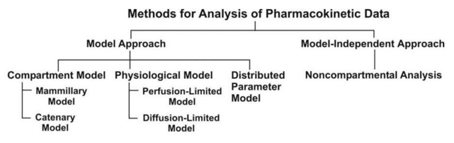
The two major approaches in the quantitative study of various kinetic processes of drug disposition in the body are (see Fig. 2) –

• Model approach, and
• Model-independent approach (also called as non-compartmental analysis).

A. Pharmacokinetic Model Approach

Pharmacokinetic models provide concise means ofexpressing mathematically or quantitatively, the time course of drug(s) throughout the body and compute meaningful pharmacokinetic parameters.

Applications of Pharmacokinetic Models –

Pharmacokinetic models are useful in —

1. Characterizing the behaviour of drugs in patients.
2. Predicting the concentration of drug in various body fluids with any dosage regimen.
3. Predicting the multiple-dose concentration curves from single dose experiments.
4. Calculating the optimum dosage regimen for individual patients.
5. Evaluating the risk of toxicity with certain dosage regimens.
6. Correlating plasma drug concentration with pharmacological response.
7. Evaluating the bioequivalence/bioinequivalence between different formulations of the same drug.
8. Estimating the possibility of drug and/or metabolite(s) accumulation in the body.
9. Determining the influence of altered physiology/disease state on drug ADME.
10. Explaining drug interactions.

Types of Pharmacokinetic Models
Pharmacokinetic models are of three different types –
1. Compartment models –are also called as empirical models, and
2. Physiological models –arerealistic models.
3. Distributed parameter models –are alsorealistic models.

1. Compartment Models

Since compartments are hypothetical in nature, compartment models are based on certain assumptions –

1. The body is represented as a series of compartments arranged either in series or parallel to each other, that communicate reversibly with each other.
2. Each compartment is not a real physiologic or anatomic region but a fictitious or virtual one and considered as a tissue or group of tissues that have similar drug distribution characteristics (similar blood flow and affinity).

Compartment Type	Perfusion Rate	Representative Tissues	Role in Model
Central	High (Instant)	Blood, Liver, Kidneys, Lungs	Administration, Elimination, Fast Distribution
Peripheral	Low (Slow)	Muscle, Skin	Intermediate Distribution
Deep	Very Low	Fat, Bone, Cartilage	Slow Distribution/Accumulation

This assumption is necessary because if every organ, tissue or body fluid that can get equilibrated with the drug is considered as a separate compartment, the body will comprise of infinite number of compartments and mathematical description of such a model will be too complex.

3. Within each compartment, the drug is considered to be rapidly and uniformly distributed i.e. the compartment is well-stirred.
4. The rate of drug movement between compartments (i.e. entry and exit) is described by first-order kinetics.
5. Rate constants are used to represent rate of entry into and exit from the compartment.

Depending upon whether the compartments are arranged parallel or in a series, compartment models are divided into two categories —

• Mammillary model-parallel
• Catenary model-series

Mammillary Model

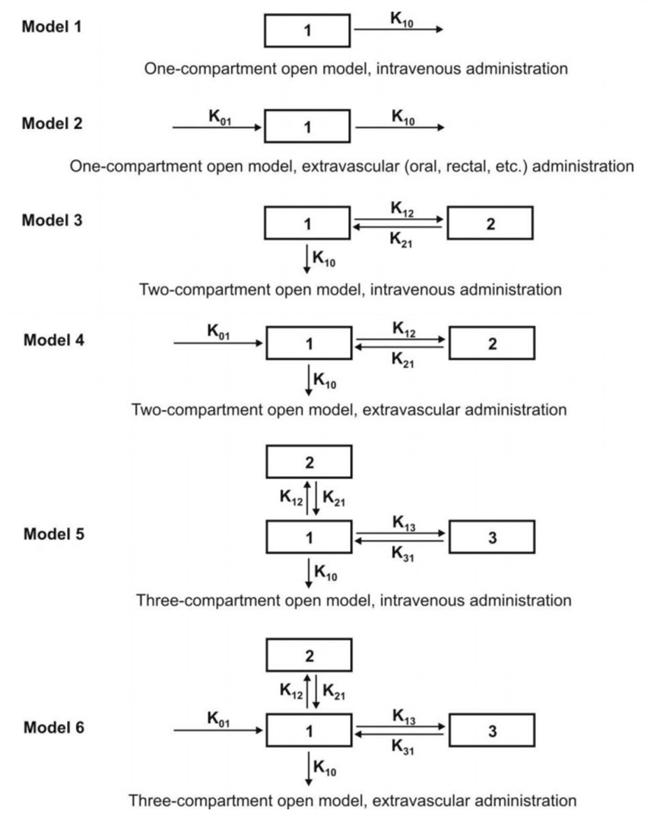
• This model is the most common compartment model used in pharmacokinetics. It consists of one or more peripheral compartments connected to the central compartment in a manner similar to connection of satellites to a planet (i.e. they are joined parallel to the central compartment).
• The central compartment (or compartment 1) comprises of plasma and highly perfused tissues such as lungs, liver, kidneys, etc. which rapidlyequilibrate with the drug. The drug is directly absorbed into this compartment (i.e. blood). Elimination too occurs from this compartment since the chief organs involved in drug elimination are liver and kidneys, the highly perfused tissues and therefore presumed to be rapidly accessible to drug in the systemic circulation.
• The peripheral compartments or tissue compartments (denoted by numbers 2, 3, etc.)are those withlow vascularity and poor perfusion. Distribution of drugs to these compartments isthrough blood.
• Movement of drug between compartments is defined by characteristic first-order rate constants denoted by letter K (see Fig. 3). The subscript indicates the direction of drug movement; thus, K₁₂ (K-one-two) refers to drug movement from compartment 1 to compartment 2 and reverse for K₂₁.

Catenary Model

In this model, the compartments are joined to one another in a series like compartments of a train (Fig. 4). This is however not observable physiologically/anatomically as the various organs are directly linked to the blood compartment. Hence this model is rarely used.

The compartment modelling approach has several advantages and applications —

1. It is often considered as “First model”. Basically, prime use of this approach is for explanation of the mass balancing of drug in plasma, drug available in the extravascular tissue and the amount of drug eliminated after its administration.
2. It gives a visual representation of various rate processes involved in drug disposition.
3. It shows how many rate constants are necessary to describe these processes.
4. It enables the pharmacokinetic scientist to write differential equations for each of the rate processes in order to describe drug-concentration changes in each compartment.
5. With limited data, It enables monitoring of drug concentration change with time. Only plasma concentration data or urinary excretion data is sufficient.
6. It is useful in predicting drug concentration-time profile in both normal physiological and in pathological conditions.
7. It is important in the development of dosage regimens.
8. It is useful in relating plasma drug levels to therapeutic and toxic effects in the body.
9. It is particularly useful when several therapeutic agents are compared. Clinically, drug data comparisons are based on compartment models.
10. Its simplicity allows for easy tabulation of parameters such as V_d, t_½, etc.

Disadvantages of compartment modelling include —

1. The compartments and parameters bear no relationship with the physiological functions or the anatomic structure of the species; several assumptions have to be made to facilitate data interpretation.
2. Extensive efforts are required in the development of an exact model that predicts and describes correctly the ADME of a certain drug.
3. The model may vary within a study population.
4. The drug behaviour within the body may fit different compartmental models depending upon the route of administration.
5. Difficulties generally arise when using models to interpret the differences between results from human and animal experiments.

Because of the several drawbacks of and difficulties with the classical compartment modelling, newer approaches have been devised to study the time course of drugs in the body. They are — physiological models and noncompartmental methods.

2. Physiological Models

• These models are also known as physiologically-based pharmacokinetic models (PB-PK models).
• They are drawn on the basis of known anatomic and physiological data and thuspresent a more realistic picture of drug disposition in various organs and tissues. 
• The number of compartments to be included in the model depends upon the disposition characteristics of the drug. 
• Organs or tissues such as bones that have no drug penetration are excluded.
• Since describing each organ/tissue with mathematic equations makes the model complex, tissues with similar perfusion properties are grouped into a single compartment. For example, lungs, liver, brain and kidney are grouped as rapidly equilibrating tissues (RET) while muscles and adipose as slowly equilibrating tissues (SET). Fig. 5 shows such a physiological model where the compartments are arranged in a series in a flow diagram.

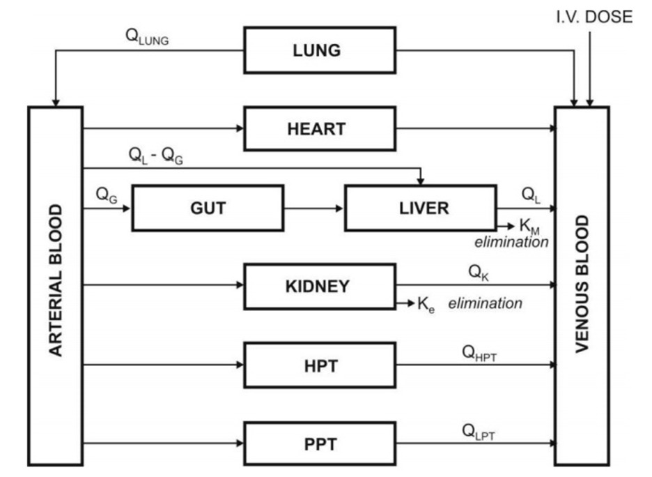
• Since it’s a physiological based model, the rate of drug carried to a tissue organ and tissue drug uptake are dependent upon two major factors –
  • Rate of blood flow to the organ, and
  • Tissue/blood partition coefficient or diffusion coefficient of drug that governs its tissue permeability.

The physiological models are further categorized into two types –

1. Blood flow rate-limited models –

• These models are more popular and commonlyused than the second type (membrane permeation rate-limited model), and are based on the assumption that the drug movement within a body region is directly proportional to its rate of delivery to that region by the perfusing blood. 
• These models are therefore also called as perfusion rate-limited models. This assumption is however applicable only to thehighly membrane permeable drugs i.e. low molecular weight, poorly ionised and highly lipophilic drugs, for example, thiopental, lidocaine, etc.

2. Membrane permeation rate-limited models –

• These models are more complexand applicable to highly polar, ionised and charged drugs, in which case the cell membrane acts as a barrier for the drug that gradually permeates by diffusion.
• These models are therefore also called as diffusion-limited models. Owing to the time lag in equilibration between the blood and the tissue, equations for these models are very complicated.

Physiological modelling has several advantages over the conventional compartment modelling 

1. Mathematical treatment is straightforward.
2. Since it is a realistic approach, the model is suitable where tissue drug concentration and binding are known.
3. Data fitting is not required since drug concentration in various body regions can be predicted on the basis of organ or tissue size, perfusion rate and experimentally determined tissue-to-plasma partition coefficient.
4. The model gives exact description of drug concentration-time profile in any organ or tissue and thus better picture of drug distribution characteristics in the body.
5. This method is frequently used in animals because invasive methods can be used to collect tissue samples.
6. Correlation of data in several animal species is possible and with some drugs, can be extrapolated to humans since tissue concentration of drugs is known.
7. Mechanism of ADME of drug can be easily explained by this model.

Disadvantages of physiological modelling include —

1. Obtaining the experimental data is a very exhaustive/lengthy process.
2. Most physiological models assume an average blood flow for individual subjects and hence prediction of individualized/personalized dosing is difficult as different individuals have different blood flow rate.
3. The number of data points is less than the pharmacokinetic parameters to be assessed.
4. Monitoring of drug concentration in body is difficult since exhaustive/lengthy data is required means needs more time.

Comparison of features of compartment and physiological models

Compartment Modelling	Physiological Modelling
Hypothetical/empirical approach – no relation with real physiology or anatomy	Realistic approach since it is based on physiological and anatomic information.
Experimentally simple and flexible approach as far as data collection is concerned	Difficult experimentally since exhaustive data collection is required.
Owing to its simplicity, it is widely used and is often the ―first model.	Less commonly used owing to complexity.
Complex multiexponential mathematical treatment is necessary for curve fitting.	Mathematical treatment is straightforward.
Data fitting is required for predicting drug concentration in a particular compartment.	Data fitting is not necessary since drug concentration in various tissues is practically determined.
Used when there is little information about the tissues.	Used where tissue drug concentration and binding are known.
Easy to monitor time course of drug in body with limited data.	Exhaustive data is required to monitor time course of drug in body.
Extrapolation from data to humans and vice versa is not possible.	Extrapolation of animal data to humans is easy on the basis of tissue concentration of drugs.
Mechanism of drug’s ADME cannot be explained.	Easy to explain drug’s ADME mechanisms.
Effect of pathological condition on drug ADME cannot be determined.	Effect of pathology on drug ADME can be easily determined.
Frequently used for data comparison of various drugs.	Less commonly used for data comparisons.

B. Noncompartmental Analysis

• The noncompartmental analysis, also called as the model-independent method, does not require the assumption of specific compartment model. This method is, however, based on the assumption that the drugs or metabolites follow linear kinetics, and on thisbasis, this technique can be applied to any compartment model.
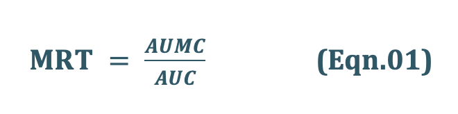
• The noncompartmental approach, based on the statistical moments theory, involvescollection of experimental data following a single dose of drug. If one considers the time course of drug concentration in plasma as a statistical distribution curve, then:

where
MRT = mean residence time
AUMC = area under the first-moment curve
AUC = area under the zero-moment curve
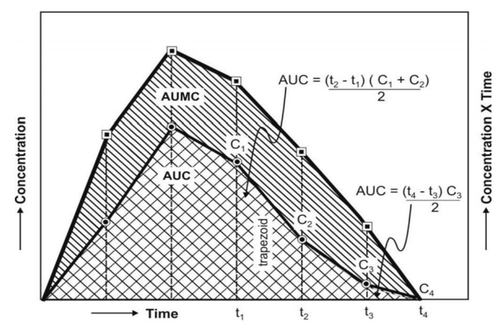
AUMC is obtained from a plot of product of plasma drug concentration versus time (i.e. C.t) versus time t from zero to infinity (Fig. 6). Mathematically, it is expressed by (integration) equation:

AUC is obtained from a plot of plasma drug concentration versus time from zero to infinity. Mathematically, it is expressed by equation:

Practically, the AUMC and AUC can be calculated from the respective graphs by the trapezoidal rule (the method involves dividing the curve by a series of vertical lines intoa number of trapezoids, calculating separately the area of each trapezoid and adding them together).

MRT (Mean residence time) is defined as the average amount of time spent by the drug in the body before being eliminated. In this sense, it is the statistical moment analogy of half-life, t_½. Ineffect, MRT represents the time for 63.2% of the intravenous bolus dose to be eliminated. The values will always be greater when the drug is administered in a fashion other than i.v. bolus.

Applications of noncompartmental technique includes–

1. It is widely used to estimate the important pharmacokinetic parameters like bioavailability, clearance and apparent volume of distribution.
2. The method is also useful in determining half-life, rate of absorption and first-order absorption rate constant of the drug.

Advantages of noncompartmental method include—

1. Ease of derivation of pharmacokinetic parameters by simple algebraic equations.
2. The same mathematical treatment can be applied to almost any drug or metabolite provided they follow first-order kinetics.
3. A detailed description of drug disposition characteristics is not required.

Disadvantages of this method include–

1. It provides limited information regarding the plasma drug concentration-time profile. More often, it deals with averages.
2. The method does not adequately treat non-linear cases.

ONE-COMPARTMENT OPEN MODEL- (Instantaneous Distribution Model)

The one-compartment open model is the simplest model based on following assumptions –

1. The body is considered as a single, kinetically homogeneous unit that has no barriers to the movement of drug.
2. Final distribution equilibrium between the drug in plasma and other body fluids (i.e. mixing) is attained instantaneously and maintained at all times. This model thusapplies only to those drugs that distribute rapidly throughout the body.
3. Drugs move dynamically, in (absorption) and out (elimination) of this compartment.
4. Elimination is a first-order (monoexponential) process with first-order rate constant.
5. Rate of input (absorption) > rate of output (elimination).
6. Concentration of drug in plasma is directly proportional to concentration of drug in all body tissues.

The term open indicates that the input (availability) and output (elimination) are unidirectional and that the drug can be eliminated from the body. Fig. 7shows such a one-compartment model. One-compartment open model is generally used to describe plasma levels following administration of a single dose of a drug.

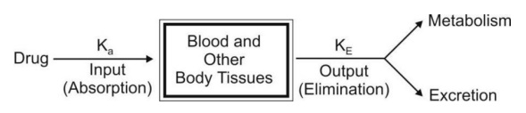
Depending upon the rate of input, several one-compartment open models can be defined:

• One-compartment open model, i.v. bolus administration.
• One-compartment open model, continuous i.v. infusion.
• One-compartment open model, e.v. administration, zero-order absorption.
• One-compartment open model, e.v. administration, first-order absorption.

One-Compartment Open Model- Intravenous Bolus Administration

• When a drug that distributes rapidly in the body is given in the form of a rapid intravenous injection (i.e. i.v. bolus or slug), it takes about one to three minutes for complete circulation and therefore the rate of absorption is neglected in calculations. The model can be depicted as follows:

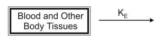
The general expression for rate of drug presentation to the body is

Since, rate in or absorption is absent, the equation becomes:

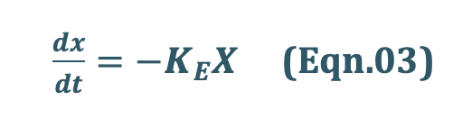
If the rate out or elimination follows first-order kinetics, then:

where,
K_E = first-order elimination rate constant, and
X = amount of drug in the body at any time t remaining to be eliminated.
Negative sign indicates that the drug is being lost from the body.

• Estimation of Pharmacokinetic Parameters

When we observe a plasma concentration time profile of a drug In i.v injection, there is no absorption phase, there is only a elimination phase. Elimination phase can be characterized by 3 parameters—

1. Elimination rate constant (K_E)
2. Elimination half-life (t_1/2)
3. Clearance (Cl).

1. Elimination Rate Constant (K_E): 

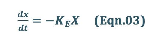
Integration of eqn.3 yields:

where,

X_o = amount of drug at time t = zero i.e. the initial amount of drug injected.
Equation Eqn. 4 can also be written in the exponential form as:

The above equation shows that disposition of a drug that follows one-compartment kinetics is monoexponential.

Transforming equation Eqn. 4 into common logarithms (log base 10), we get:

Since it is difficult to determine directly the amount of drug distributed in all organs/tissues in the body X, advantage is taken of the fact that a constant relationship exists between drug concentration in plasma C (easily measurable) and X; thus:

Hence, we can use C instead X. The equation Eqn.06 therefore becomes:

where,
C_o = plasma drug concentration immediately after i.v. injection.
Eqn. 8 is that of a straight line and indicates that a semilogarithmic plot of log C versus t will be linear with Y-intercept log C_o. 
The elimination rate constant is directly obtained from the slope of the line (Fig. 8b). It has units of min^–1. Thus, a linear plot is easier to handle mathematically than a curve which in this case will be obtained from a plot of C versus t on regular (Cartesian) graph paper (Fig. 8a).

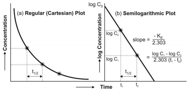
Thus, C_o, K_E (and t_½) can be readily obtained from log C versus t graph. 

2. Elimination Half-Life:

Also called as biological half-life. It is defined as the time taken for the amount of drug in the body as well as plasma concentration to decline by one-half or 50% its initial value. It is expressedin hours or minutes. Half-life is related to elimination rate constant by the following equation:

Elimination half-life can be readily obtained from the graph of log C versus t as shown in Fig 8.

The half-life is a secondary parameter that depends upon the primary parameters clearance and apparentvolume of distribution according to following equation:

We know that, 

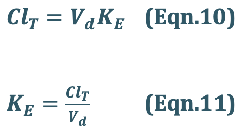
Substitute Eqn. 11 into Eqn. 09
Hence Eqn. 09 will be, 

3. Clearance: 

Clearance is defined as the theoretical volume of body fluid containing drug(i.e. thatfraction of apparent volume of distribution) from which the drug is completely removed in a given period of time. It is expressed in ml/min or liters/hour.

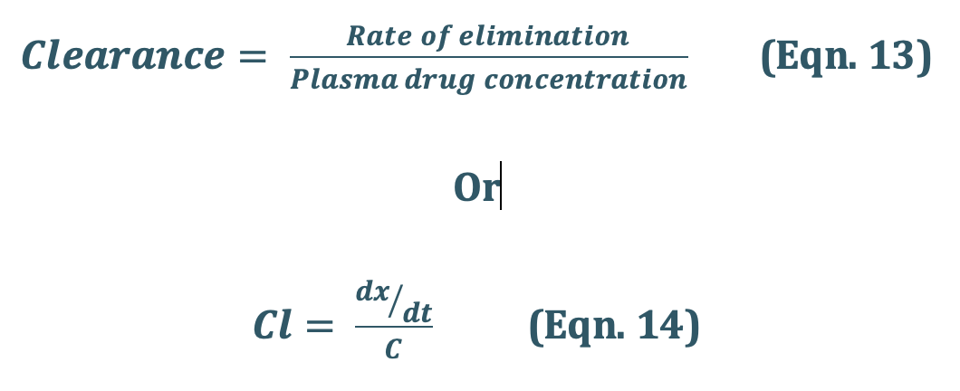
Total Body Clearance: Elimination of a drug from the body involves processes occurringin kidney, liver, lungs and other eliminating organs. Clearance at an individual organ level is called as organ clearance. It can be estimated by dividing the rate of elimination by eachorgan with the concentration of drug presented to it. Thus,

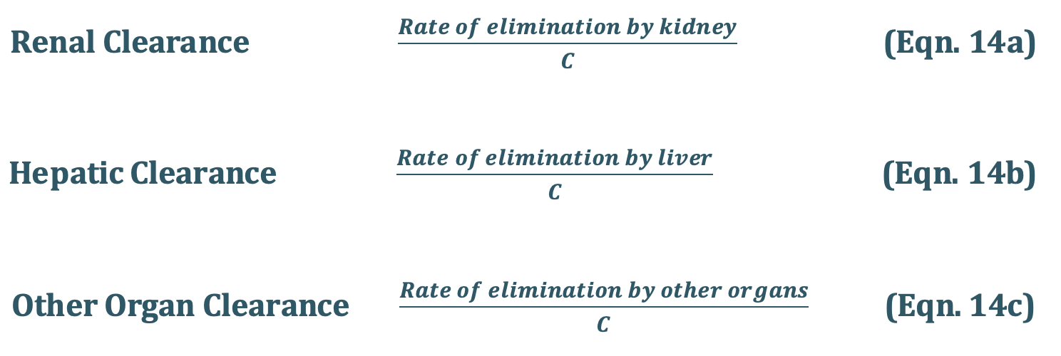
The total body clearance, Cl_T, also called as total systemic clearance, is an additive property of individual organ clearances. Hence,
Total Systemic Clearance

---

One-Compartment Open Model- Intravenous Infusion

Rapid i.v. injection (bolus) is unsuitable when the drug has potential to cause toxicity or when maintenance of a stable concentration or amount of drug in the body is desired. In such a situation, the drug is administered at a constant rate (zero-order) by i.v. infusion. 

Advantages of zero-order infusion of drugs include—

1. Ease of control of rate of infusion to fit individual patient needs.
2. Prevents fluctuation between maximum safe concentration and minimum effective concentration, desired especially when the drug has a narrow therapeutic index.
3. Other drugs, electrolytes and nutrients can be conveniently administered simultaneously by the same infusion line in critically ill patients.

Types of cases:

1. Case I – Normal i.v infusion.
2. Case II – Steady state concentration achieved through i.v infusion.
3. Case III – Steady state concentration achieved with Loading dose (i.v bolus + i.v infusion)

In this i.v infusion, the pharmacokinetic parameter considered is concentration of drug in the blood.

1. Case I – Normal i.v infusion.

The model can be represented as follows:

At any time during infusion, the rate of change in the amount of drug in the body, dX/dt is the difference between the zero-order rate of drug infusion R_o and first-order rate of elimination, –K_EX:

Integration and exponential rearrangement of above equation yields:

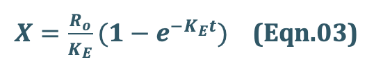
We know, X = V_d C
Since X = V_d C, the Eqn.03 can be transformed into concentration terms as follows:

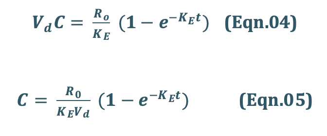
Since Cl_T, = K_EV_d = the above equation becomes,

2. Case II – Steady state concentration achieved through i.v infusion.

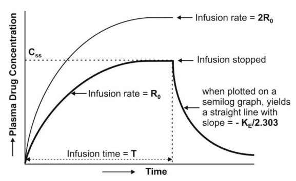
At the start of constant rate infusion, the amount of drug in the body is zero and hence, there is no elimination. As time passes, the amount of drug in the body rises gradually (elimination rate less than the rate of infusion) until a point after which the rate of elimination equals the rate of infusion i.e. the concentration of drug in plasma approaches a constant value called as steady-state, plateau or infusion equilibrium (Fig. 9).

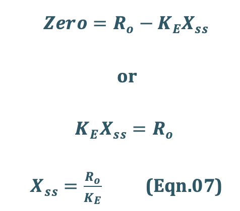
At steady-state, the rate of change of amount of drug in the body is zero, hence, the equation 

Eqn.02 becomes:

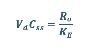
Since, X = V_d C, then the X_ss = V_d C_ss,

Substitute X_ss = V_d C_ss in Eqn.07

Transforming to concentration terms and rearranging the equation:

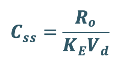
Since, Cl_T = K_E V_d, substitute Cl_T value in above equation.

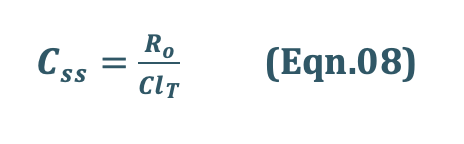
where, X_ss and C_ss are amount of drug in the body and concentration of drug in plasma at steady-state respectively. The value of K_E (and hence t_½) can be obtained from the slope of straight line obtained after a semilogarithmic plot (log C versus t) of the plasma concentration-time data gathered from the time when infusion is stopped (Fig. 9.3). Alternatively, K_E can be calculated from the data collected during infusion to steady-state as follows:

Consider case I concentration final equation,

Substituting R_o/Cl_T = C_ss from Eqn.08 into Eqn.09 we get:

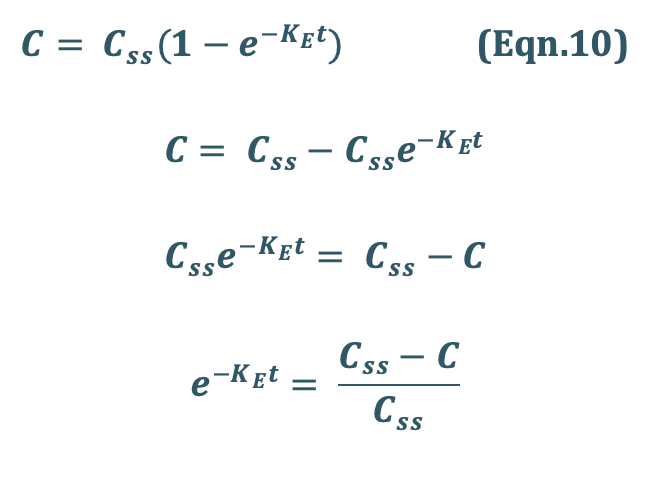
Rearrangement yields:

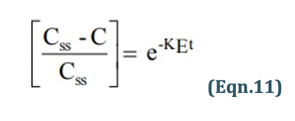
Transforming into log form, the equation becomes:

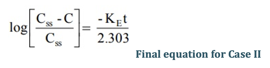
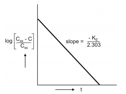
A semilog plot of (C_ss – C)/C_ss versus t results in a straight line with slope –K_E/2.303 (Fig. 10).

3. Case III – Steady state concentration achieved with Loading dose (i.v bolus + i.v infusion)

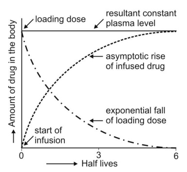
Infusion Plus Loading Dose: It takes a very long time for the drugs having longer half-lives before the plateau concentration is reached (e.g. phenobarbital, 5 days). Thus, initially, such drugs have subtherapeutic concentrations. This can be overcome by administering an i.v. loading dose large enough to yield the desired steady-state immediately upon injection prior to starting the infusion. It should then be followed immediately by i.v. infusion at a rate enough to maintain this concentration (Fig. 11).

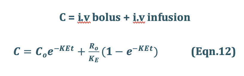
Recalling once again the relationship X = V_dC, the equation for computing the loading dose X_o,L can be given:

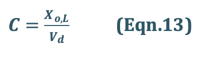
Substitution of Eqn.13 into Eqn.12 yields another expression for loading dose in terms of infusion rate:

Assessment of Pharmacokinetic Parameters

where, T = infusion time.
The above equation is a general expression which can be applied to several pharmacokinetic models.

---

One-Compartment Open Model – Extravascular Administration

• When a drug is administered by extravascular route (e.g. oral, i.m., rectal, etc.), absorption is a prerequisite for its therapeutic activity.
• The rate of absorption may be described mathematically as a zero-order or first-order process.
• A large number of plasma concentration-time profiles can be described by a one-compartment model with first-order absorption and elimination. 
• However, under certain conditions, the absorption of some drugs may be better described by assuming zero-order (constant rate) kinetics. Differences between zero-order and first-order kinetics are illustrated in Fig. 12.

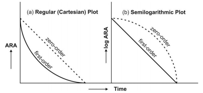
Zero-order absorption is characterized by a constant rate of absorption. It is independentof amount remaining to be absorbed (ARA), and its regular ARA versus t plot is linear with slope equal to rate of absorption while the semilog plot is described by an ever-increasing gradient with time. In contrast, the first-order absorption process is distinguished by a decline in the rate with ARA i.e. absorption rate is dependent upon ARA; its regular plot is curvilinear and semilog plot a straight line with absorption rate constant as its slope.

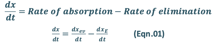
• After e.v. administration, the rate of change in the amount of drug in the body dX/dt is the difference between the rate of input (absorption) dX_ev/dt and rate of output (elimination) dX_E/dt.

• For a drug that follows one-compartment kinetics, the plasma concentration-time profile is characterized by absorption phase, post-absorption phase and elimination phase (Fig. 13).

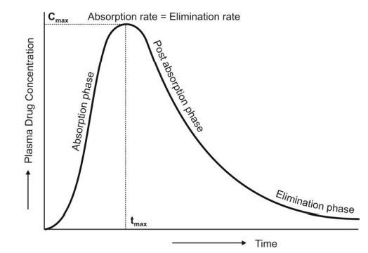
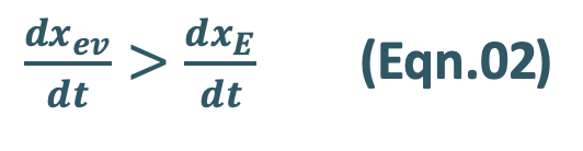
• During the absorption phase, the rate of absorption is greater than the rate of elimination

• At peak plasma concentration, the rate of absorption equals the rate of elimination and the change in amount of drug in the body is zero.

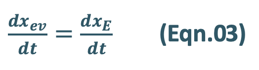
• During the post-absorption phase, there is some drug at the extravascular site still remaining to be absorbed and the rate of elimination at this stage is greater than the absorption rate.

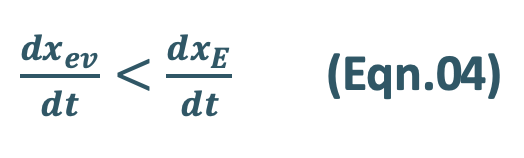
• After completion of drug absorption, its rate becomes zero and the plasma level time curve is characterized only by the elimination phase.

a. Zero-Order Absorption Model

This model is similar to that for constant rate infusion.

The rate of drug absorption, as in the case of several controlled drug delivery systems, is constant and continues until the amount of drug at the absorption site (e.g. GIT) is depleted. All equations that explain the plasma concentration-time profile for constant rate i.v. infusion are also applicable to this model.

b. First-Order Absorption Model

For a drug that enters the body by a first-order absorption process, gets distributed in the body according to one-compartment kinetics and is eliminated by a first-order process, the model can be depicted as follows:

The differential form of the Eqn.01 is:

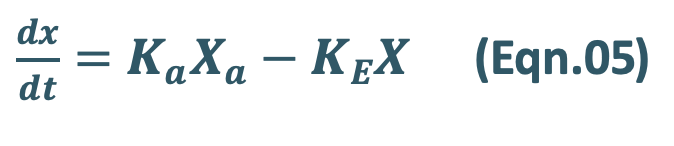
where, 
K_a = first-order absorption rate constant, and
X_a = amount of drug at the absorption site remaining to be absorbed i.e. ARA.

Integration of Eqn.05 yields:

Since we know 
X = V_d C, then C = X/V_d

 Transforming into concentration terms, the equation becomes:

Where, F = fraction of drug absorbed systemically after e.v. administration. A typical plasma concentration-time profile of a drug administered e.v. is shown in Fig. 13.

---